Big O Complexities
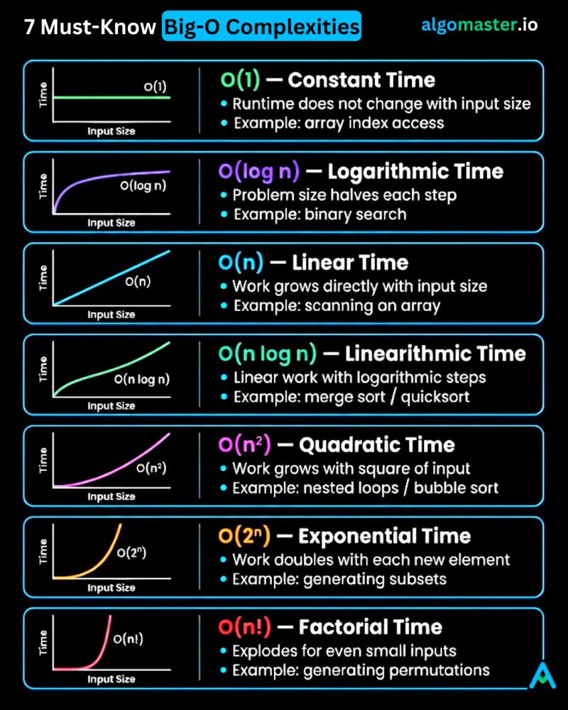
1. 𝐎(1) – 𝐂𝐨𝐧𝐬𝐭𝐚𝐧𝐭 𝐭𝐢𝐦𝐞 - The runtime doesn't change regardless of the input size. - Example: Accessing an element in an array by its index.
2. 𝐎(𝐥𝐨𝐠 𝐧) – 𝐋𝐨𝐠𝐚𝐫𝐢𝐭𝐡𝐦𝐢𝐜 𝐭𝐢𝐦𝐞 - The runtime grows slowly as the input size increases. Typically seen in algorithms that divide the problem in half with each step. - Example: Binary search in a sorted array.
3. 𝐎(𝐧) – 𝐋𝐢𝐧𝐞𝐚𝐫 𝐭𝐢𝐦𝐞 - The runtime grows linearly with the input size. - Example: Finding an element in an array by iterating through each element.
4. 𝐎(𝐧 𝐥𝐨𝐠 𝐧) – 𝐋𝐢𝐧𝐞𝐚𝐫𝐢𝐭𝐡𝐦𝐢𝐜 𝐭𝐢𝐦𝐞 - The runtime grows slightly faster than linear time. It involves a logarithmic number of operations for each element in the input. - Example: Sorting an array using quick sort or merge sort.
5. 𝐎(𝐧^2) – 𝐐𝐮𝐚𝐝𝐫𝐚𝐭𝐢𝐜 𝐭𝐢𝐦𝐞 - The runtime grows proportionally to the square of the input size. - Example: Bubble sort algorithm which compares and potentially swaps every pair of elements.
6. 𝐎(2^𝐧) – 𝐄𝐱𝐩𝐨𝐧𝐞𝐧𝐭𝐢𝐚𝐥 𝐭𝐢𝐦𝐞 - The runtime doubles with each addition to the input. These algorithms become impractical for larger input sizes. - Example: Generating all subsets of a set.
7. 𝐎(𝐧!) – 𝐅𝐚𝐜𝐭𝐨𝐫𝐢𝐚𝐥 𝐭𝐢𝐦𝐞 - Runtime is proportional to the factorial of the input size. - Example: Generating all permutations of a set.